


![[Guest Post] Survival of the Savviest: Actionable Website Strategies for Small Businesses in Tough Times](https://static.wixstatic.com/media/24bff7_9eaf5fe147aa45dfad5f848a9d30ef96~mv2.png/v1/fill/w_604,h_604,fp_0.50_0.50,q_35,blur_30,enc_avif,quality_auto/24bff7_9eaf5fe147aa45dfad5f848a9d30ef96~mv2.png)
![[Guest Post] Survival of the Savviest: Actionable Website Strategies for Small Businesses in Tough Times](https://static.wixstatic.com/media/24bff7_9eaf5fe147aa45dfad5f848a9d30ef96~mv2.png/v1/fill/w_148,h_148,fp_0.50_0.50,q_95,enc_avif,quality_auto/24bff7_9eaf5fe147aa45dfad5f848a9d30ef96~mv2.png)


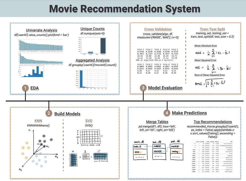
How to Build a Collaborative Based Filtering Movie Recommendation System
- Visual Design Studio

- Dec 6, 2021
- 7 min read
Updated: Feb 1, 2022
A Beginner Friendly Guide to Recommender System
Recommender system has become a rising topic as we demand more customized contents push to our daily feeds. I guess we are all familiar with the recommended videos on YouTube, and we are all - more than once - the victims of late-night Netflix binge watching.
There are two popular methods in recommender system, collaborative based filtering and content based filtering. Content based filtering makes predictions of what the audience is likely to prefer based on the content properties, e.g. genre, language, video length. Whereas collaborative filtering predicts based on what other similar users also prefer. As the result, collaborative filtering method is leaning towards instance based learning and usually applied by large companies with huge amount of data at hand.
In this article, I will focus on collaborative based filtering and briefly introduce how to make movie recommendation using two algorithms that fall into this category, K Nearest Neighbour (KNN) and Singular Value Decomposition (SVD).
I used the movie dataset from Kaggle to predict recommended movies for each individual. Let's first load the ratings table into a dataframe.
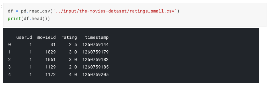
If you would like to access the full code of this exercise, please visit the Code Snippet section.
📊 EDA for Recommender System
Each machine learning algorithm requires different way to explore the dataset to get valuable insights. I performed following three techniques to explore the data at hand. To see a more comprehensive guide of EDA, please have a look at this blog: Semi-Automated Exploratory Data Analysis Process in Python.
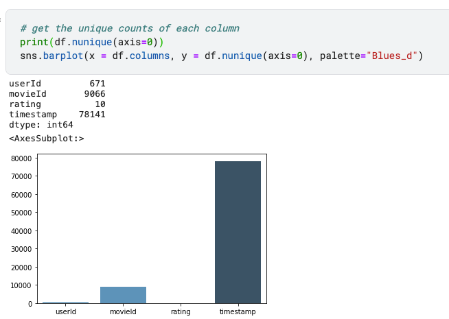
1. Unique Counts and Data Shape
Firstly, an overview of how many distinct users and movies are included in the dataset. This can be easily achieved using df.nunique(axis = 0) and then plot it in a bar chart.
2. Univariate Analysis
Univariate analysis - the analysis of one feature at a time, helps us to better understand three questions:
what are the movies with most reviews?
who are the users that provide most reviews?
how does the distribution looks like for ratings?
# univariate analysis
plt.figure(1, figsize = (16,4))
df['movieId'].value_counts()[:50].plot(kind = 'bar') #take top 50 movies
plt.figure(2, figsize = (16,4))
df['userId'].value_counts()[:50].plot(kind = 'bar') #take top 50 users
plt.figure(3, figsize = (8,4))
df['rating'].plot(kind = 'hist')
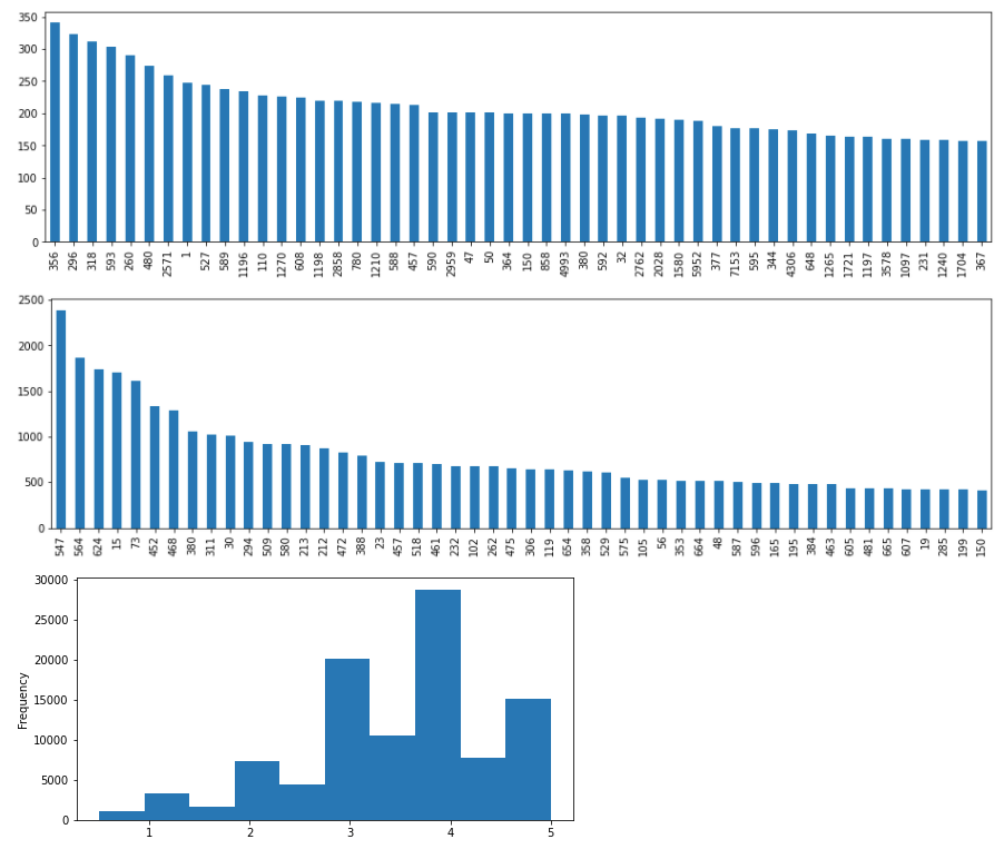
Some of the insights we can draw from these distribution charts are:
1. ratings are not evenly distributed among movies and the most rated movies is "356" which has no more than 350 ratings;
2. ratings are not evenly distributed across users and users at most provided around 2,400 ratings;
3. most people are likely to give a rating around 4
3. Aggregated Analysis
Univariate analysis gives us a view more at individual movies or users level, whereas aggregated analysis helps us to understand the data on the meta-level.
1. What is the distribution of ratings given to each movie? - the histogram shows that most users (roughly 560 out of 671 - 80%) fall into the range of 0-250 ratings
ratings_per_user = df.groupby('userId')['movieId'].count() ratings_per_user.hist() 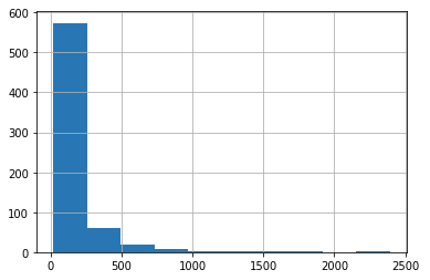
2. What is the distribution of users who provide ratings? - the histogram shows that most movies (roughly 8,200 out of 9,066 - 90%) have less than 25 ratings
ratings_per_movie = df.groupby('movieId')['userId'].count() ratings_per_movie.hist() 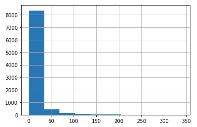
At this stage, we should have a fairly clear understanding of the data at hand.
💻 Collaborative -Based Filtering Algorithms
I would like to introduce two collaborative based filtering algorithms - K nearest neighbor and Singular value decomposition. The surprise library in python allows us to implement both algorithms in just several lines of code.
from surprise import KNNWithMeans
from surprise import SVD

# k Nearest Neighbour
similarity = {
    "name": "cosine",
    "user_based": False,  # item-based similarity
}
algo_KNN = KNNWithMeans(sim_options = similarity)


# SVD
algo_SVD = SVD()
But it's always better to have a basic knowledge of the theory behind each algorithm in order to implement it appropriately. To understand the algorithms better, we may need to transform the ratings dataframe into a userId by movieId matrix format.
movie_rating_set = pd.crosstab(index = df.userId, columns = df.movieId, values = df.rating, aggfunc = np.mean)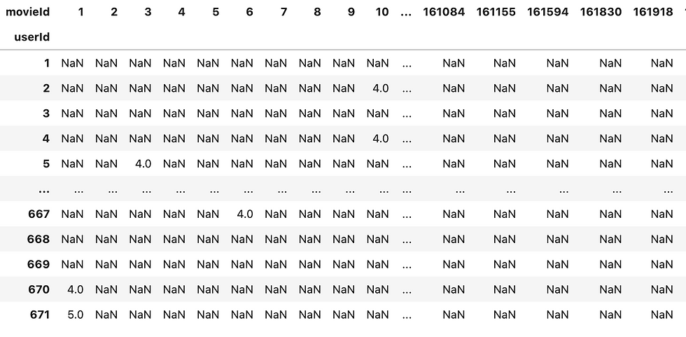
1. K Nearest Neighbour (KNN)
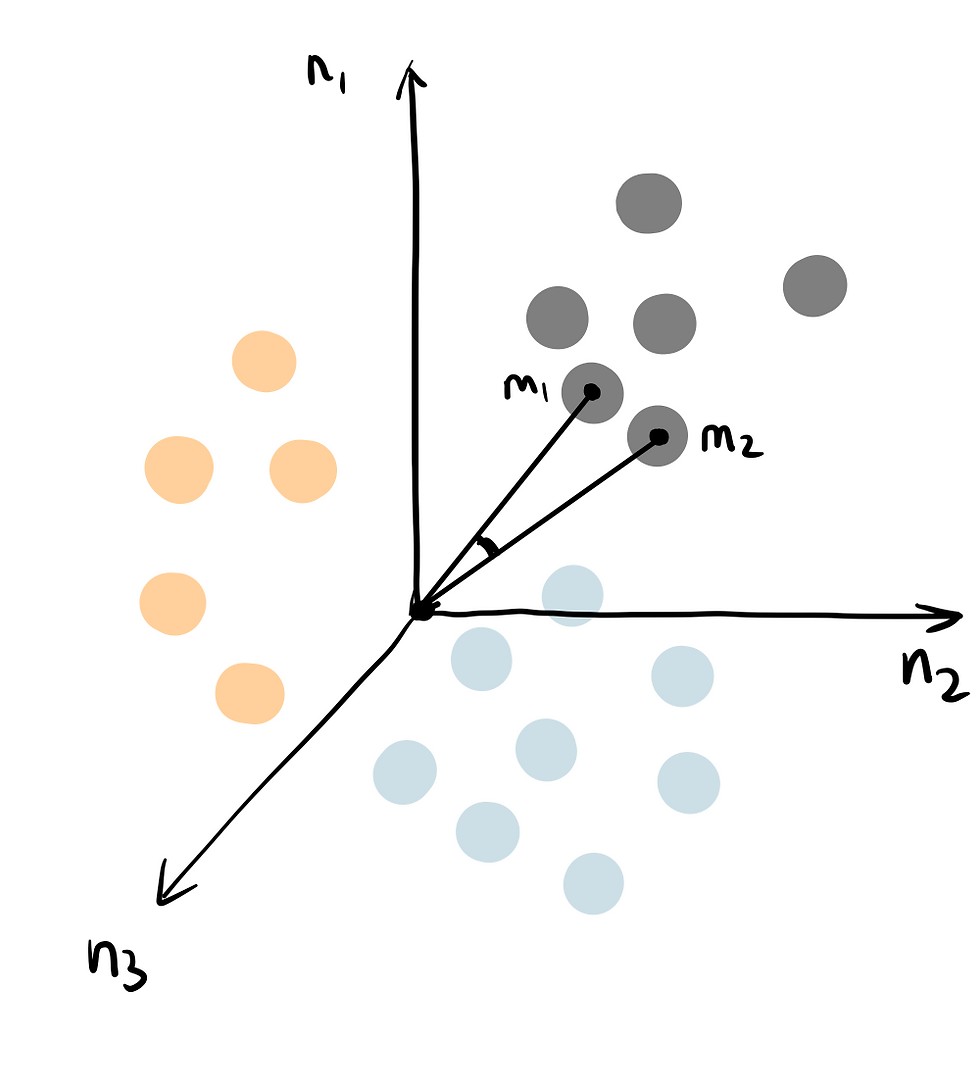
The option user_based: False determines that this KNN uses item-based similarity, so that we are predicting the unknown ratings of item m1 based on similar items with known ratings. You can think of k nearest neighbour algorithm as representing movie items in a n dimensional space defined by n users. The distance among points are calculated based on cosine similarity - which is determined by the angle between two vectors (as shown m1 and m2 in the diagram). Cosine similarity is preferred instead of Euclidean distance, because it suffers less when the dataset is high in dimensionality.
2. Matrix Factorization - Singular Value Decomposition (SVM)
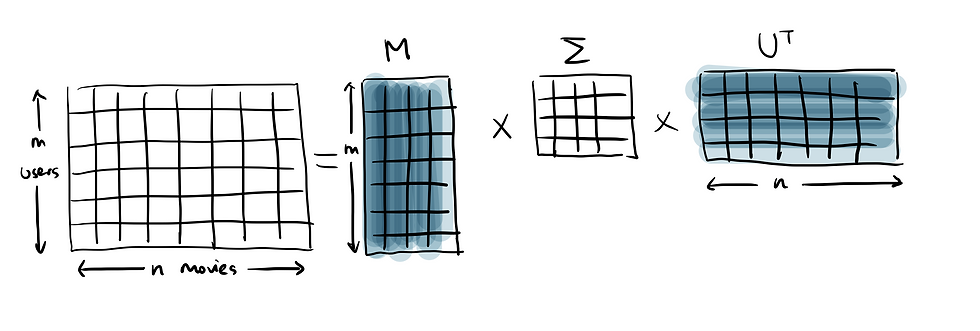
Singular value decomposition is a matrix factorization technique that decomposes the matrix into the product of lower dimensionality matrices, and then extracts the latent features from highest importance to lowest. I know it is quite a long sentence, so let me break it down.
Instead of iterating through individual ratings like KNN, it views the rating matrix as a whole. Therefore, it has less computation cost compared to KNN but also makes it has less interpretability.
SVD extract the latent features (which is not an actual features contained in the dataset, but what the algorithm magically discovered as valuable hidden features) to form the factorized matrices U and V transposed, and placed them in a descending feature importance order. It then fills in the blank ratings taking the product of U and V transposed in a weighted approach based on feature importance. These latent feature parameters are learned iteratively through minimizing the cost function. And this brings us to the next section - model evaluation.
Model Evaluation
Collaborative filtering technique represents recommender system as a regression supervised model, where the output is a numeric rating value. So we can apply regression evaluation metrics to our recommendation system. If you would like to dive deeper into evaluation metrics for regression, e.g. linear regression, you may find the model evaluation section in the "A Simple and Practical Guide to Linear Regression" helpful.
In this exercise, I evaluate both KNN and SVD in following two methods.
1. Cross Validation
Surprise library offers a built-in cross_validate function that executes cross validation automatically. Firstly, ingest the dataset into Surprise Reader object using load_from_df and then keep the rating scale between 0 and 5.
from surprise import Dataset
from surprise import Reader

# load df into Surprise Reader object
reader = Reader(rating_scale = (0,5))
rating_df = Dataset.load_from_df(df[['userId', 'movieId', 'rating']], reader)
Secondly, pass both algo_KNN and algo_SVD into the cross_validate function with 5 cross validation folds.
## Method 1. cross validation ##
from surprise.model_selection import cross_validate
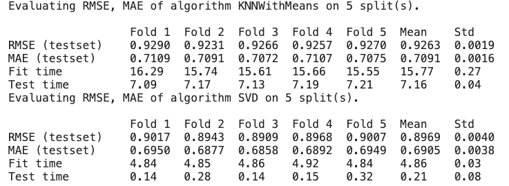
cross_validate_KNN = cross_validate(algo_KNN, rating_df, measures=['RMSE', 'MAE'], cv=5, verbose=True)
cross_validate_SVD = cross_validate(algo_SVD, rating_df, measures=['RMSE', 'MAE'], cv=5, verbose=True)The result shows the comparison between KNN and SVD. As shown, SVD has smaller RMSE, MAE values, hence performs better than SVD, and also takes significantly less time to compute.
2. Simple Train-Test Split
## Method 2. build training and testing set ##
from surprise.model_selection import train_test_split
from surprise import accuracy

# define train test function
def train_test_algo(algo, label):
    training_set, testing_set = train_test_split(rating_df, test_size = 0.2)
    algo.fit(training_set)
    test_output = algo.test(testing_set)
    test_df = pd.DataFrame(test_output)

    print("RMSE -",label, accuracy.rmse(test_output, verbose = False))
    print("MAE -", label, accuracy.mae(test_output, verbose=False))
    print("MSE -", label, accuracy.mse(test_output, verbose=False))

    return test_df
This approach splits dataset into 80% for training and 20% for testing. Instead of iterating the model build 5 times as in cross validation, it will only train the model and test it once. The function train_test_algo also prints out RMSE, MAE, MSE and return the test dataframe.
Let's compare the model accuracy and have a glimpse of the test output.
# get test result
train_test_KNN = train_test_algo(algo_KNN, "algo_KNN")
print(train_test_KNN.head())

train_test_SVD = train_test_algo(algo_SVD, "algo_SVD")
print(train_test_SVD.head())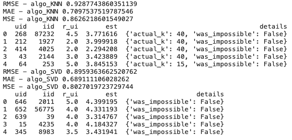
The result is very similar to the cross validation, indicating that SVD has less error.
🎞 Provide Top Recommendation
It is not enough just building the model. As you can see above, the current test output only predicts ratings for userId and movieId randomly allocated to the test set. We need to see the actual recommendation with movie names.
Firstly, let's load the movie metadata table and links table, so that we can translate movieId into movie name.
# load movie data and links data
movie_df = pd.read_csv("../input/the-movies-dataset/movies_metadata.csv")
links_df = pd.read_csv("../input/the-movies-dataset/links.csv")
movie_df['imdb_id'] = movie_df['imdb_id'].apply(lambda x: str(x)[2:].lstrip("0"))
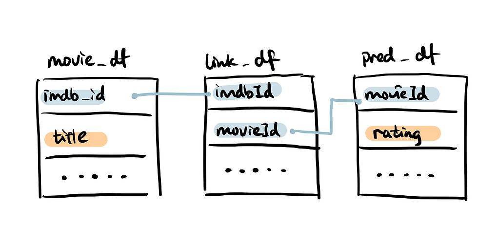
links_df['imdbId'] = links_df['imdbId'].astype(str)
Here is a diagram of how three dataframes link together.
Then I defined a prediction(algo, users_K) function that allows you to create a dataframe for K number of users that you are interested in and iterate through all 9067 movies in the dataset while calling the recommendation algorithm.
def prediction(algo, users_K):
    pred_list = []
    for userId in range(1,users_K):
        for movieId in range(1,9067):
            rating = algo.predict(userId, movieId).est
            pred_list.append([userId, movieId, rating])
    pred_df = pd.DataFrame(pred_list, columns = ['userId', 'movieId', 'rating'])
    return pred_df
Lastly, top_recommendations(pred_df, top_N) function performs following procedure:
1) merges the dataset together using pd.merge();
2) group the ratings by userId and sort it by rating value in a descending order;
3) get the top values using head();
4) return both the sorted recommendations and the top recommended movies
def top_recommendations(pred_df, top_N):
    link_movie = pd.merge(pred_df, links_df, how='inner', left_on='movieId', right_on='movieId')
    recommended_movie = pd.merge(link_movie, movie_df, how='left', left_on='imdbId', right_on='imdb_id')[['userId', 'movieId', 'rating', 'movieId','imdb_id','title']]
    sorted_df = recommended_movie.groupby(('userId'), as_index = False).apply(lambda x: x.sort_values(['rating'], ascending = False)).reset_index(drop=True)
    top_recommended_movies = sorted_df.groupby('userId').head(top_N)
    return sorted_df, top_recommended_movies
As a side note, when apply merge in dataframe, we need to be more mindful of datatype of the keys that are joined together, or else you will get a lot of empty result.
Lastly, compare the top 3 predictions given by the KNN vs. SVD.
# KNN predictions
pred_KNN = prediction(algo_KNN, 10)
recommended_movies_KNN, top_recommended_movies_KNN = top_recommendations(pred_KNN, 3)

## SVD predictions
pred_SVD = prediction(algo_SVD, 10)
recommended_movies_SVD, top_recommended_movies_SVD = top_recommendations(pred_SVD, 3)
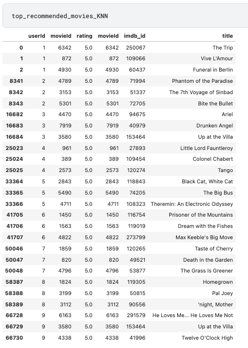

As you can see two algorithms give different recommendations and KNN appears to be much more generous in terms of ratings.
Hope you enjoy this article and thanks for reaching this far. If you would like to access the full code or contribute by signing up premium membership, please visit our Code Snippet.
Take-Home Message
This article takes you through the procedure of building a recommender system and compare the recommendations provided by KNN vs. SVD.
A top-line summary:
EDA for Recommender System: univariate analysis, aggregated analysis
Two Collaborative Based Filtering Algorithm: K Nearest Neighbour vs. Singular Value Decomposition
Model Evaluation: cross validation vs. train-test split
Provide Top Recommendations


Comments